The first PID loop I tuned in production was a furnace outlet temperature controller on a gas-to-liquids facility in Africa. I’d been taught Ziegler-Nichols at university, and I tried to apply it on a real process during commissioning. It worked, sort of. The loop oscillated more than the operations team was comfortable with, the integral action was too aggressive, and within two days a senior engineer had retuned it using something he called “lambda tuning.”
His version held setpoint smoothly, rejected disturbances cleanly, and the operators stopped calling control room about it.
That was the moment I learned the gap between what’s taught and what’s used. PID tuning methods are an academic discipline with decades of theoretical literature, but in oil and gas, refining, and chemical process industries, practitioners use a much smaller set of approaches than the textbooks cover. Different methods suit different loop types. Some methods are taught everywhere but rarely deployed in production.
This guide walks through the PID tuning methods that matter in practice — what each one does, when it’s actually used, and which methods experienced engineers reach for first. I’ve tuned loops on Honeywell Experion PKS, Yokogawa CENTUM, and Emerson DeltaV across multiple oil and gas projects. The vendor changes the tools but not the underlying tuning principles.
If you’ve read our What Is a DCS cornerstone guide, this article goes one level deeper into the actual loop tuning work that engineers do during commissioning and ongoing optimization.
TL;DR — Quick Answer: What Are PID Tuning Methods?
PID tuning methods are systematic approaches for setting the three controller parameters — proportional gain (Kp), integral time (Ti), and derivative time (Td) — so a PID loop achieves stable, responsive control of a process variable. The main methods include Ziegler-Nichols, Cohen-Coon, Lambda Tuning, Internal Model Control (IMC), Skogestad’s rules (SIMC), and manual heuristic tuning.
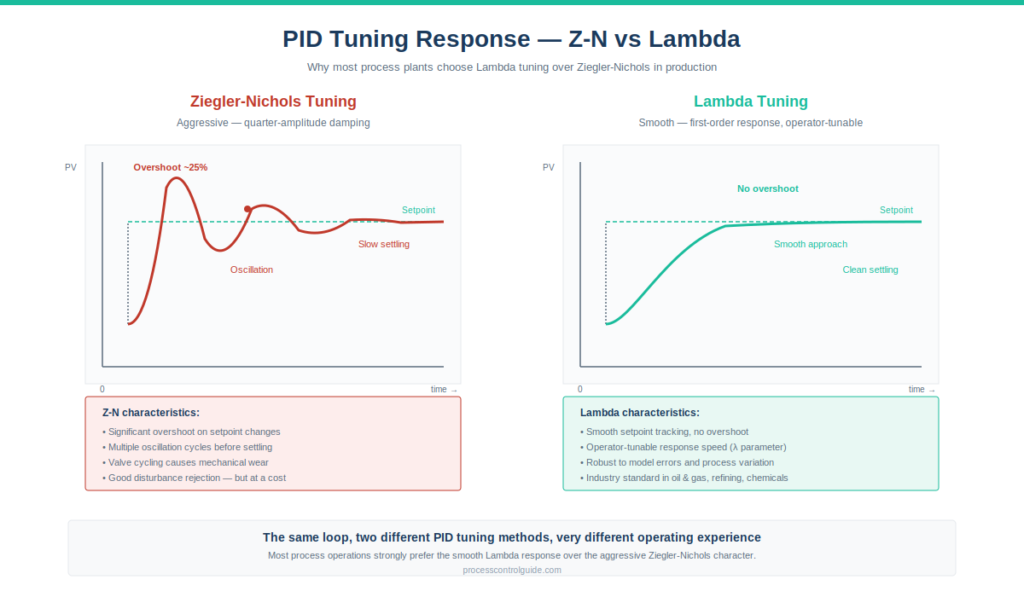
Different methods optimize for different objectives. Ziegler-Nichols was the first systematic method (1942) and produces aggressive tuning suitable for disturbance rejection but with significant overshoot. Cohen-Coon improves on Z-N for processes with significant dead time. Lambda tuning is the most widely used method in chemical, refining, and oil and gas industries because it produces smooth, robust control with operator-tunable response speed.
In modern industrial practice, the two PID tuning methods that dominate are Lambda tuning and manual heuristic tuning. Auto-tuners built into vendor DCS platforms (Honeywell Loop Scout, Emerson DeltaV InSight, Yokogawa Exaplog) provide computer-assisted tuning for engineers who don’t want to do the math by hand. Different loop types — flow, pressure, level, temperature — call for different tuning strategies regardless of the method chosen.
What You Will Learn
This guide covers PID tuning methods at the depth working engineers actually need:
- What PID tuning means and why it matters in real plants
- Ziegler-Nichols (closed-loop and open-loop variants) — what it is and why it’s rarely used in process industries today
- Cohen-Coon — when this older method still applies
- Lambda Tuning — the modern industry-standard approach explained
- Internal Model Control (IMC) — Lambda’s mathematical cousin
- Manual heuristic tuning — what most engineers actually do
- Vendor-specific auto-tuners on Experion, CENTUM, and DeltaV
- How loop type (flow, pressure, level, temperature) drives method selection
- Common PID tuning mistakes from real projects
What Is PID Tuning — A Working Definition
PID tuning methods are systematic approaches for selecting numerical values for the three controller parameters that make a closed-loop control system stable and well-behaved. PID stands for Proportional-Integral-Derivative — the three terms that combine to produce a controller output based on the error between setpoint and measurement.
The three parameters are:
- Proportional gain (Kp) — how strongly the controller reacts to current error
- Integral time (Ti) — how strongly the controller reacts to accumulated past error
- Derivative time (Td) — how strongly the controller reacts to the rate of change of error
Tuning means choosing these three numbers correctly for the specific process being controlled. Get them right and the loop tracks setpoint smoothly, rejects disturbances quickly, and runs without operator complaints. Get them wrong and the loop either oscillates wildly, responds too slowly, or stays in a permanent steady-state error.
PID tuning methods exist because process dynamics vary enormously. A flow loop has fast dynamics with little dead time. A temperature loop on a large vessel has slow dynamics with significant dead time. A level loop on a knockout drum has integrating dynamics that behave differently from self-regulating processes. The same Kp, Ti, Td values that work beautifully on one loop type will completely fail on another.
The ISA standards catalog contains educational materials and standards related to controller tuning, and most major DCS vendors publish their own tuning guidance documents. The international PID controller algorithm is also formally defined in IEC 61131-3, the standard governing programmable controllers used in industrial automation.
Why PID Tuning Methods Matter in Process Plants
A well-tuned PID loop is invisible — the result of carefully chosen PID tuning methods applied during commissioning and refined over time. It tracks setpoint, rejects disturbances, and operators forget it exists. A poorly tuned PID loop is the opposite — it oscillates, alarms, requires constant operator intervention, and eventually gets put in manual mode where it stays for months.
The business consequences of bad tuning compound over time:
- Production losses — oscillating loops produce off-spec product, trigger interlocks, or fail to maintain target rates
- Equipment wear — aggressive tuning cycles valves and actuators constantly, accelerating mechanical wear
- Operator burden — loops in manual mode require constant operator attention that drains time from real problems
- Safety implications — loops that don’t respond well to disturbances can drift toward trip setpoints and cause spurious shutdowns
- Energy costs — temperature loops that overshoot waste fuel; flow loops that hunt waste pumping energy
On every major project I’ve been on, the application of appropriate PID tuning methods directly correlates with operations satisfaction and plant performance. A modern process plant might have 1,000+ PID loops across the BPCS. The engineering effort to tune them well is significant — but the engineering effort to live with badly tuned loops over a 30-year plant life is far greater.
The Main PID Tuning Methods — An Overview
There are six PID tuning methods worth knowing for process industry work:
| Method | Year | Best For | Industry Use |
|---|---|---|---|
| Ziegler-Nichols | 1942 | Disturbance rejection, simple processes | Rare in chemical/oil & gas; common in education |
| Cohen-Coon | 1953 | Processes with significant dead time | Occasional; mostly superseded |
| Lambda Tuning | 1968 | Smooth setpoint tracking, robust control | Industry standard in refining and chemicals |
| IMC (Internal Model Control) | 1980s | Model-based design | Common in academic and advanced applications |
| Skogestad’s Rules (SIMC) | 2001 | Simplified model-based tuning | Growing adoption in industry |
| Manual Heuristic | always | New loops, troubleshooting | Universal — every engineer uses this |
Each of these PID tuning methods has its place. In practice, most experienced process engineers reach for Lambda or manual heuristic tuning for routine work, with occasional use of Cohen-Coon on dead-time-dominant loops and the others reserved for specialized situations or educational reference.
Ziegler-Nichols Tuning Method
Ziegler-Nichols is the most famous PID tuning method, developed by John Ziegler and Nathaniel Nichols at Taylor Instruments in 1942. It’s the method everyone learns in university, and it’s the method most engineers stop using once they enter industry.
The Z-N method has two variants:
Closed-Loop (Ultimate Sensitivity) Method.
This is the original Z-N approach. The procedure is:
- Put the controller in Automatic with only proportional action (Ti and Td disabled)
- Make a small setpoint change and observe the response
- Gradually increase the proportional gain (Kp) until the loop just begins to oscillate with constant amplitude
- Record the proportional gain at this point — this is the “ultimate gain” Ku
- Measure the period of oscillation — this is the “ultimate period” Pu
- Calculate PID parameters from standard formulas: Kp = 0.6 × Ku, Ti = Pu/2, Td = Pu/8
The result is an aggressively tuned controller that quarter-amplitude damps — meaning each oscillation cycle has roughly 1/4 the amplitude of the previous one.
Open-Loop (Reaction Curve) Method.
The open-loop variant doesn’t require driving the process to instability. Instead:
- Put the controller in Manual
- Make a small step change in controller output
- Record the process variable response over time
- Identify the process characteristics: dead time (L), time constant (T), and process gain (K) from the reaction curve
- Calculate PID parameters from Z-N formulas based on L, T, and K
The result is again aggressive tuning suitable for disturbance rejection.
Why Z-N is rarely used in industry today.
Z-N tuning produces aggressive response with significant overshoot, which is acceptable in some applications but problematic in most chemical and oil and gas processes. The 25% quarter-amplitude damping criterion that Z-N targets is too oscillatory for plants that need stable, smooth operation.
Additionally, the closed-loop method requires deliberately driving the process to the edge of instability — something nobody wants to do on a running production unit. The open-loop variant is safer but still produces aggressive tuning that doesn’t match what modern plants want.
In my career, I’ve used Z-N once or twice as a starting point on a new loop where I had no idea what to expect — but I’ve never finalized a loop in Z-N tuning. The aggressive response is just not what process operations wants.
Cohen-Coon Tuning Method
Cohen-Coon is one of the older PID tuning methods, developed by G.H. Cohen and G.A. Coon in 1953, specifically to improve on Ziegler-Nichols for processes with significant dead time. The method uses the same open-loop reaction curve test as Z-N, but applies different formulas designed for systems where dead time dominates the process dynamics.
The Cohen-Coon procedure:
- Conduct an open-loop step test, identical to Z-N open-loop method
- Identify process gain (K), dead time (L), and time constant (T) from the reaction curve
- Apply Cohen-Coon formulas, which adjust the tuning based on the L/T ratio
The math is more involved than Z-N because the formulas explicitly account for the ratio of dead time to time constant. For processes where L is significant compared to T (sometimes called “lag-dominated” processes), Cohen-Coon typically produces better results than Z-N.
Where Cohen-Coon still applies.
Cohen-Coon is occasionally useful when:
- The process has high dead time relative to time constant (long pipe runs, large transport lags)
- A formal model-based method isn’t available
- Quick-start tuning is needed and Z-N would be too aggressive
But among modern industrial PID tuning methods, Cohen-Coon has been largely superseded by Lambda tuning. The Lambda approach handles dead-time-dominant processes well while also providing a tunable parameter for the desired closed-loop response speed — something Cohen-Coon doesn’t offer.
Lambda Tuning — The Industry Standard
Lambda tuning is the most widely used PID tuning method in chemical processing, refining, and oil and gas industries today. It was first proposed by Dahlin in 1968 and developed into industrial practice over subsequent decades, particularly through work at companies like ExxonMobil and Foxboro.
The core idea is straightforward: instead of optimizing for aggressive disturbance rejection like Z-N, design the controller to produce a desired closed-loop response speed (the “lambda”) that the engineer chooses based on what the plant actually needs.
The Lambda procedure:
- Conduct an open-loop step test to identify process gain (K), dead time (L), and time constant (T)
- Choose lambda (λ) — the desired closed-loop time constant
- Apply Lambda formulas: Kp = T / (K × (λ + L)), Ti = T, Td = 0 for PI control (Lambda is typically applied as PI rather than full PID)
The lambda choice is the key engineering decision that distinguishes Lambda from other PID tuning methods. A small lambda (faster than the process time constant) produces aggressive response. A larger lambda (slower than process time constant) produces conservative, smooth response.
Why Lambda dominates in process industries.
Lambda tuning has several practical advantages:
- Operator-tunable response speed — the lambda parameter directly controls how fast the loop responds. Want smoother control? Increase lambda. Want faster response? Decrease lambda. This is intuitive and adjustable.
- Robust to model errors — Lambda tuning is forgiving of imperfect process identification. A 20 percent error in identified time constant doesn’t ruin the tuning.
- Predictable behavior — Lambda produces well-defined closed-loop response (essentially first-order plus dead time), which operators can understand and predict.
- Excellent for setpoint tracking — Lambda excels at smooth setpoint changes without overshoot, which matches what most process operations want.
For practitioner-oriented coverage of Lambda tuning and related methods, ControlGuru is one of the most respected industrial process control resources online and goes into significantly more mathematical depth than this guide.
Lambda trade-off.
Lambda tuning generally produces weaker disturbance rejection than aggressive methods like Z-N. For loops that experience significant disturbances and need to recover quickly, Lambda may not be the best choice. Modified Lambda variants address this in specific cases.
In my own experience tuning loops on Experion, CENTUM, and DeltaV, Lambda tuning is the method I reach for first on any new loop where I have time to do a proper step test. It produces consistently good results across temperature loops on furnaces, pressure loops on separators, and flow loops on feedstock systems.
For broader DCS context where loops live, see our Honeywell Experion PKS architecture guide and Yokogawa CENTUM VP architecture guide.
Internal Model Control (IMC) Tuning
Internal Model Control is one of the model-based PID tuning methods developed in the 1980s, primarily through academic work at Caltech and the University of California. The approach is mathematically similar to Lambda tuning but is presented in a different framework based on explicit process model identification.
The IMC procedure:
- Identify a process model (typically first-order plus dead time or second-order plus dead time)
- Choose a filter time constant (similar to Lambda’s lambda parameter)
- Derive PID parameters analytically from the model and filter constant
The relationship to Lambda is direct — for many process model structures, IMC and Lambda tuning produce essentially identical PID parameters. The methods differ more in pedagogical framing than in mathematical outcome.
Where IMC stands in practice.
IMC tuning is widely taught in academic process control courses and appears in vendor literature as the basis for some auto-tuner implementations. In hands-on industrial practice, engineers tend to use Lambda terminology and Lambda procedures even when the underlying math is IMC. The two approaches converge in working tools.
Skogestad’s Rules (SIMC) — The Modern Simplification
Sigurd Skogestad at NTNU in Norway published the “SIMC” PID tuning method (Simple Internal Model Control) tuning rules in 2001, providing a simplified version of IMC tuning that’s easier to apply by hand. SIMC has gained significant industrial adoption in the 25 years since. The original Skogestad SIMC paper remains freely available from NTNU and is the authoritative reference.
The SIMC approach gives explicit formulas for PI and PID tuning based on first-order plus dead time and integrating processes, with a single tuning parameter (typically taken as the closed-loop time constant). The formulas are simple enough to apply mentally or with a quick calculation.
SIMC is increasingly the recommended approach in modern process control courses and texts. For practitioners, it offers the rigor of model-based tuning with the simplicity of rule-based tuning — a useful middle ground.
Manual Heuristic Tuning — What Most Engineers Actually Do
Despite all the systematic PID tuning methods above, the most common approach in industry is manual heuristic tuning. This means putting the controller in service with reasonable starting values, observing how it behaves, and adjusting parameters by feel based on experience.
The classical heuristic approach:
- Start with conservative Kp, large Ti, zero Td
- Make a small setpoint change and observe the response
- If response is too slow, increase Kp gradually
- If response oscillates, decrease Kp or increase Ti
- Repeat until response is acceptable
- Add derivative action only if needed (rare on most loops)
This sounds primitive, but in the hands of experienced engineers it produces excellent results faster than formal step tests. The reason is that experienced engineers carry a mental model of how different loop types should respond — a flow loop should look like this, a temperature loop on a furnace should look like that, a level loop on a knockout drum should behave this way. They tune to that mental model rather than calculating from formulas.
When manual heuristic tuning is the right choice.
- Quick fixes during operations when formal step tests aren’t practical
- Troubleshooting loops that have drifted from previous tuning
- New loops with limited downtime windows for step testing
- Loops where the dynamics are too variable for any fixed model to capture
- Final fine-tuning after applying a formal method as a starting point
In my own work, I almost always apply one of the formal PID tuning methods first (usually Lambda) to get a reasonable starting point, then manually adjust based on how the loop actually behaves with real process disturbances. The formal method gets you 80 percent of the way; manual heuristic adjustment closes the last 20 percent that matters for operator acceptance.
Vendor-Specific PID Auto-Tuners
Modern DCS platforms include built-in PID tuning methods through auto-tuners that automate the step test and parameter calculation process. These tools have become significantly more capable over the past decade and are increasingly used in industry.
Honeywell Experion PKS — Loop Scout / Loop Performance Solutions.
Loop Scout is Honeywell’s loop monitoring and tuning solution, integrated with Experion PKS. It can identify poorly performing loops, suggest tuning improvements, and in some configurations apply auto-tuning. On the oil and gas mega-project in Asia where I currently work, Loop Scout is used for ongoing loop performance monitoring across the BPCS.
Yokogawa CENTUM VP — Exaplog and Tuning Tools.
Yokogawa’s CENTUM VP includes built-in tuning utilities within the engineering environment. The Exaplog platform provides ongoing loop performance monitoring, and step-test-based auto-tuning is available as part of the standard toolset.
Emerson DeltaV — InSight and Tune.
DeltaV InSight is Emerson’s loop monitoring and analytics package. The DeltaV Tune feature provides built-in auto-tuning capability using step tests run directly from the engineering workstation. The tool covers PI and PID tuning with options for different tuning rules.
For deeper DeltaV context, see our Emerson DeltaV architecture guide.
Honest assessment of auto-tuners.
Modern auto-tuners produce good starting points but rarely produce the final tuning that goes into production. Most engineers I work with treat the auto-tuner output as a baseline and then apply manual adjustments based on actual loop behavior. The combination of formal PID tuning methods (auto-tuner running Lambda or IMC) plus manual fine-tuning is the typical workflow.
Loop Type Matters — Different Strategies for Different Loops
The same PID tuning methods applied uniformly to every loop will produce poor results because process dynamics vary dramatically across loop types. Experienced engineers carry different mental templates for different loops.
Flow Loops.
Flow loops have fast dynamics, minimal dead time, and clean self-regulating response. Tuning is typically:
- Proportional gain modest (often 0.5 to 2)
- Integral time short (5 to 30 seconds)
- Derivative time zero (derivative action is generally not used on flow loops because of noise on flow measurement)
Flow loops are the easiest to tune. Almost any method produces acceptable results.
Pressure Loops.
Pressure loops on liquid systems behave like fast self-regulating processes similar to flow. Pressure loops on gas systems can have integrating dynamics if the vessel is large. Tuning depends on the underlying physics:
- Liquid pressure: tune like flow loops
- Gas pressure on small vessels: similar to flow with slightly longer integral time
- Gas pressure on large vessels: integrating process tuning required (different formulas)
Level Loops.
Level loops are pure integrating processes — there’s no self-regulation from the process itself. Lambda tuning has specific integrating-process formulas that differ from self-regulating processes. The common mistake is tuning level loops with self-regulating formulas, which produces sluggish recovery from disturbances.
Many level loops on buffer tanks should be tuned slowly on purpose — the tank exists to absorb upstream disturbances, and tight level control defeats this purpose. Loose level tuning with significant proportional band is often the right answer.
Temperature Loops.
Temperature loops are the slowest in most plants. Process time constants of minutes to tens of minutes are typical. Dead time can be significant depending on sensor location and process volumes.
Lambda tuning works well on temperature loops when proper step tests can be conducted. For temperature loops with significant disturbances (furnaces, reactors), cascade control with secondary fast loops is often more effective than pure feedback tuning regardless of method.
For a complete practitioner guide to cascade architecture and tuning, see our Cascade Control Explained guide.
Common PID Tuning Mistakes I’ve Seen
After applying various PID tuning methods on loops across multiple vendor platforms, here are the recurring mistakes:
Using Z-N tuning on real process loops. Z-N produces aggressive quarter-amplitude damping that doesn’t match what modern process operations wants. The method survives in education but should be rare in production tuning.
Identical tuning across different loop types. A flow loop tuned with temperature-loop parameters will respond too slowly to be useful. Temperature loops tuned with flow-loop parameters will oscillate. Different loop types need different approaches even within the same tuning method.
Adding derivative action everywhere. Derivative action is genuinely useful on a small minority of loops — slow temperature loops with clean signals, mainly. On flow loops, pressure loops, and most level loops, derivative amplifies measurement noise and creates more problems than it solves. The vast majority of process loops should be PI, not PID.
Tuning during commissioning then never revisiting. Process dynamics change over plant life. Heat exchangers foul, valves wear, instrumentation drifts. Tuning that was perfect at commissioning may be marginal three years later. Periodic loop performance review catches this drift.
Ignoring valve and actuator dynamics. A loop tuned aggressively will exercise the control valve constantly. If the valve has significant stiction or backlash, the loop will hunt. Sometimes the right answer isn’t more aggressive tuning but mechanical valve maintenance.
Trusting auto-tuner output without verification. Auto-tuners produce mathematically valid tuning for the model they identified. If the identified model is wrong (incomplete step test, disturbances during the test, nonlinear process), the resulting tuning will be wrong. Always validate auto-tuner output by observing actual loop behavior.
Tuning to setpoint changes only, ignoring disturbance response. A loop can look beautiful on setpoint step tests and perform poorly on actual disturbances. Tune for the dominant operating mode — if the loop mostly rejects disturbances rather than tracking setpoints, tune for disturbance rejection.
Forgetting filter settings. Most modern DCS platforms apply input filtering on measurements. Filter time constants too short produce noisy controller output. Filter time constants too long add effective dead time to the loop. Filter selection interacts with PID tuning and needs to be considered together.
Treating PID as the only answer. Some loops genuinely need more than PID — cascade control, feedforward control, ratio control, or model predictive control. Trying to tune a fundamentally limited PID loop into perfect performance when an additional control structure would solve the problem is wasted effort.
Frequently Asked Questions
What are the three parameters in PID tuning?
PID tuning methods all work with three controller parameters: proportional gain (Kp), integral time (Ti), and derivative time (Td). Kp controls reaction to current error, Ti controls accumulated past error correction, and Td controls reaction to rate of change of error. Most process loops use PI (no derivative); full PID is appropriate for a minority of loops.
Which PID tuning method is best?
For most process industry applications, Lambda is the preferred PID tuning method because it produces smooth, robust control with operator-tunable response speed. Manual heuristic tuning is the most commonly used approach for routine work. Ziegler-Nichols, while widely taught, is rarely used in production process plants.
Why is Ziegler-Nichols not used in industry?
Ziegler-Nichols produces aggressive tuning with significant overshoot, which is acceptable in some applications but problematic in most chemical, oil and gas, and refining processes. The closed-loop method also requires deliberately driving the process to the edge of instability — undesirable in production. Lambda tuning has largely replaced Z-N as the preferred PID tuning method in industrial practice.
What is Lambda tuning?
Lambda tuning is a PID tuning method where the engineer specifies a desired closed-loop response time (the lambda) and the PID parameters are calculated to achieve that response. Lambda tuning is the industry standard in chemical processing, refining, and oil and gas because it produces smooth, robust control with adjustable response speed.
How do I know if my PID loop is well tuned?
A well-tuned PID loop tracks setpoint with minimal overshoot, rejects disturbances quickly, and runs without operator intervention. Process oscillation, frequent operator complaints, loops put in manual mode, or excessive valve cycling all indicate tuning problems.
Should every PID loop have derivative action?
No. The vast majority of process loops should be PI rather than full PID. Derivative action amplifies measurement noise and creates problems on most loops. Derivative is genuinely useful on a small subset of slow loops with clean signals — primarily certain temperature loops.
Can I use the same PID tuning for similar loops?
Sometimes, but with caution. Two flow loops on similar pipes with similar valves may share tuning. Two temperature loops on similar vessels with similar heating may share tuning. But “similar” usually isn’t similar enough — small differences in process dynamics produce noticeable differences in tuning requirements. Better to step-test each loop than to copy tuning.
What is auto-tuning in modern DCS systems?
Auto-tuning is a software feature in modern DCS platforms (Honeywell Loop Scout, Emerson DeltaV Tune, Yokogawa Exaplog) that conducts an automated step test on a loop and calculates suggested PID parameters. Auto-tuners produce good starting points but typically require manual fine-tuning based on actual operating behavior.
How often should PID loops be retuned?
Most operating companies recommend reviewing loop performance annually and revisiting PID tuning methods on loops that have degraded. Major plant modifications, equipment replacement, or significant operational changes should trigger immediate retuning of affected loops. Some loops stay perfectly tuned for decades; others drift constantly.
Conclusion
PID tuning methods are an academic discipline with decades of theoretical development, but practical industrial tuning narrows to a smaller set of approaches. Lambda tuning dominates in chemical, refining, and oil and gas industries. Manual heuristic tuning is what experienced engineers actually do for most routine work. Ziegler-Nichols, while universally taught, sees little production use because its aggressive response doesn’t match what modern process operations need.
The best PID tuning method depends on the loop type, the process dynamics, the operational context, and the engineer’s experience level. New engineers should learn formal methods systematically. Experienced engineers blend formal methods with intuition and platform-specific tools. Auto-tuners in modern DCS platforms can accelerate the process but don’t replace engineering judgment.
The most important practical truth is that tuning isn’t a one-time activity. Process dynamics change over plant life. Valves wear, exchangers foul, instrumentation drifts, operating conditions evolve. Periodic loop performance review and retuning are part of normal plant operation — not just a commissioning activity.
If you’re new to PID tuning, start with Lambda tuning and manual heuristic adjustment. Avoid Z-N for production tuning. Always conduct step tests properly, validate auto-tuner results, and match the tuning method to the loop type. The discipline pays off in plant performance, operator satisfaction, and long-term reliability.
For broader DCS context, see our What Is a DCS cornerstone guide. For vendor-specific platform context where PID loops are configured and tuned, see our Honeywell Experion PKS architecture guide, Yokogawa CENTUM VP architecture guide, and Emerson DeltaV architecture guide.
For the practitioner treatment of how PID tuning, cascade control, and advanced process control apply to petroleum refineries — including critical control loops in CDU furnace outlet temperatures, FCC reactor temperature, hydrocracker WABT, and column tray temperatures — see our DCS in Refining guide.
About the Author
Daniel Reed is an Instrument and Controls Engineer with 14+ years of oil and gas EPC experience across onshore and offshore projects in Asia and Africa. He currently works as a client-side I&C completion engineer on a large oil and gas mega-project in Asia, where he has been involved with Honeywell Experion PKS and Safety Manager since 2018.
His earlier work covered Yokogawa CENTUM and Triconex SIS on an offshore brownfield in Africa (2015-2018), and Yokogawa CENTUM and ProSafe-RS on a gas-to-liquids facility in Africa. His focus is engineering deliverable review, control and safety system commissioning, HAZOP/SIL/SIF participation, FAT/SAT execution, loop tuning across multiple DCS platforms, and vendor coordination across Honeywell, Yokogawa, Triconex, Allen-Bradley, and Siemens platforms.